Selecting Heating, Cooling Units for High-Altitude Homes
Selecting heating and cooling equipment for high altitudes requires modified procedures to account for lower air density, usually any application at 2,500 feet or higher. This guidance is provided by the OEM and in the Air Conditioning Contractors of America’s (ACCA’s) Manual S, Selection of Residential HVAC Equipment, the reference adopted in the 2009 International Code Council Residential Building Code.
 At high altitudes the air is thinner, less dense. This thin air has less heat-carrying capacity. At sea level, 1,200 cubic feet per minute (cfm) of air can carry 36,000 Btuh. However, at 5,000 feet, the thinner air carries less heat; about 1,430 cfm are needed to carry 36,000 Btuh, as will be displayed in the example below.
When considering the effects of high-altitude HVAC installations and that more air is needed, the OEM and Manual S base their guidance on three basic principles:
1. One cfm of air is always 1 cfm, no matter what the elevation.
2. Air at high elevations is less dense and carries less heat.
 3. The density of the air depends on the elevation of the HVAC system installation.
Two other rules the HVAC system designer should remember when selecting equipment at higher elevations are:
1. Equipment capacity is determined by the OEM.
2. Only when OEM data is not available should the HVAC system designer use generic tables like the one offered in this article, ACCA Technical Bulletin 2008-01, and Manual S.


• The pressure drop across the metering orifice;
• The density of the combustion air; and
• The oxygen content of the combustion air.
This is affected by altitude. Refer to OEM guidance (specify make, model, and required options and accessories) to derate and adjust the nameplate temperature rise.
Output Capacity: To determine output capacity, first adjust input capacity, and then multiply the adjusted input capacity by the sea-level steady-state efficiency (not the AFUE) of the furnace.
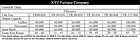
 For this example, consider a sea-level furnace that has 80,000 Btuh of input capacity and an 80 percent steady-state efficiency (See Figure 2). This furnace is considered for our example home in Denver (the specific model will be evaluated later). The OEM directs that the furnace capacity be derated 4 percent for every 1,000 feet above sea level. (This will vary based on the OEM.)
Input Btuh = 80,000 – [80,000 x (4% x 5,000 / 1,000)] = 64,000
Output Btuh = 80% x 64,000 = 51,200
Where:
4% = The OEM value to derate the furnace
5,000 = Altitude of the installation
80,000 = Input capacity of the FR 80 Series furnace
64,000 = Altitude adjusted input capacity of FR 80 Series furnace
The 80,000-Btuh furnace will have enough heating capacity of the example home (51,200 Btuh).
Temperature Rise: The temperature rise (TR) across the furnace heat exchanger is also affected by altitude. Manual J, Table 10A contains altitude correction factors (ACF) for air density at different elevations. (See Figure 3.) The ACF is applied to the formula used to calculate the TR:
TR = Btuh / (cfm x 1.1 x ACF)
 In this formula, the Btuh is the output capacity of the furnace. At sea level, an example of the TR is:
Sea-level output Btuh = 80% x 80,000 = 64,000
Sea-Level TR = (64,000) / (1.1 x 1.00 x 1,600) = 36.4°F
Where:
80% = Steady-state efficiency of the FR 80-036
80,000 = Input capacity of the FR 80 Series furnace
64,000 = Altitude adjusted input capacity of the FR 80 Series furnace
1.1 = Physics constant to convert the weight of dry air at sea level into volume
1.00 = ACF for sea level
1,600 = Airflow in cfm
After this sea-level example, what is the TR of the same furnace at altitude? Use the same 80,000-input Btuh, single-stage, 80 percent efficiency moving 1,600 cfm, but move it to Denver. Note: The nameplate TR will not change for high-altitude installations; see the OEM instructions. For this example, XYZ furnace FR 80-036, the nameplate TR is 30-60° (See Figure 2).
To calculate the TR for high altitude, first adjust the input capacity. Second, use the adjusted input capacity to determine the output capacity (adjusted for altitude). Finally, use the altitude adjusted output capacity to calculate the TR.
Value to derate the input Btuh = 80,000 x 4% x (5,000 / 1,000) = 16,000
Derated Denver input Btuh = 80,000 – 16,000 = 64,000
Derated Denver output Btuh = 64,000 x 80% = 51,200
Derated Denver TR = (51,200) / (1.1 x 0.84 x 1,600) = 34.6°F
Where (the previous factors still apply):
4% = The OEM value to derate the furnace
51,200 = Altitude adjusted output capacity of FR 80 Series furnace
0.84 = ACF for Denver (5,000 feet - See Figure 3)
1,600 = Airflow in cfm
5,000 = Altitude of the installation
A cfm of 1,600 is still 1,600 cfm at 5,000 feet. However, the unit’s capacity has been decreased because of the high elevation, the thinner air carries less heat, and the resulting temperature rise can be evaluated for design purposes. In this case, the TR margin for the new furnace is too slim; less airflow (1,200 cfm equals a more tolerable 46° TR) would serve this application better.
The equipment’s capacity is associated with a specified airflow as seen in Figure 4. This airflow becomes the design cooling airflow (if it meets the Manual D duct sizing requirements).
Our example home had a total cooling load of 30,000 Btuh (See Figure 1) - 29,000 sensible and 1,000 latent. The following 3-ton XYZ unit is considered.
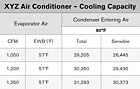
Denver’s summer (cooling) design temperature is 90°F. See Figure 5 for the interpolated capacities from the expanded performance data.
The altitude adjustment factor is 0.92 (5,000 feet, and a dry coil based on a 97 percent sensible heat ratio.) See Figure 7 for the altitude adjusted capacities for the 3-ton unit in the example.
 Based on these capacities, the 3-ton unit will meet the cooling loads; the only choice now is which blower setting to use. At 1,050 cfm, the unit is just a little short on capacity, the choice is acceptable but not the most desirable. At 1,200 cfm, the cooling capacity is acceptable, and at that airflow the TR through the furnace would be 46.2, at 1,350 the TR would be 41. Both are acceptable.
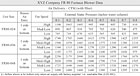
Further, after examining the FR 80-036 blower performance data (see Figure 8), it can be seen that 1,200 cfm can be achieved at 0.81 inches water column (wc) on medium-high fan speed. Using the design external static pressure should allow for the air conditioner coil, a good filter, and a standard duct system.
Fan Performance: 1,200 cfm at 0.81 external static pressure
Less 0.31 inches wc for the air conditioner coil (per XYZ Co. specs)
Less 0.25 inches wc for the pleated filter (per filter specs)
Less 0.25 inches wc for the duct system (approximately)
Total: 0.81 External static pressure
Therefore, based on the heating capacity of the FR 80-036, the cooling capacity of the AC-36, and the blower capacity of the FR80-036, the home should have the following equipment: XYZ FR80-036 furnace with an AC-36 with the AC-036 coil. The airflow for the furnace should be set on medium-high fan speed for heating and cooling. The ducts and all external accessories should create no more than 0.81 inches wc of external static pressure.
Equipment selection is a vital step in the HVAC system design process. But, equipment selection and HVAC system design are only one of the four pillars to a quality installation. The heating and cooling system may be meticulously designed, but if the equipment is improperly installed, or if the duct system is leaky, then the customer views the contractor as a bungling amateur. The solution: Design HVAC systems properly and then follow the other three pillars of a quality installation in the ACCA Quality Installation Specification, which is available for free download at www.acca.org/quality.
Publication date: 03/30/2009
WHAT'S DIFFERENT?
As a quick review of the residential HVAC design process, after calculating the home’s heating and cooling requirements, or loads, the HVAC system designer should consult Manual S and the OEM’s expanded performance data to select the best HVAC system for the customer. In this case, the best unit is the smallest unit that will heat and cool the home. There are other factors which should be considered and are very important: air filtration, humidity control (beyond normal cooling capacity), quiet operation, and many others. But these are outside the scope of Manual S.Figure 1. Manual J heating and cooling loads.
When considering the effects of high-altitude HVAC installations and that more air is needed, the OEM and Manual S base their guidance on three basic principles:
1. One cfm of air is always 1 cfm, no matter what the elevation.
2. Air at high elevations is less dense and carries less heat.
Figure 2. XYZ Furnace Company: Performance data.
Two other rules the HVAC system designer should remember when selecting equipment at higher elevations are:
1. Equipment capacity is determined by the OEM.
2. Only when OEM data is not available should the HVAC system designer use generic tables like the one offered in this article, ACCA Technical Bulletin 2008-01, and Manual S.
Figure 3. This table provides approximate correction factors for the range of air temperatures associated with comfort heating and cooling processes. Accuracy is compatible with the accuracy of load calculation procedures, equipment selection procedures, and duct design procedures. Calculations for industrial process equipment and special heating and cooling applications may require adjustment factors that consider changes in air temperature.
A SIMPLE EXAMPLE
To illustrate how to select equipment for higher elevations, consider the following simple example to select a gas furnace and air conditioner for a home in Denver. This example will use information from ACCA Manual S, ACCA Technical Bulletin 2008-01, and the OEM expanded performance data. The example home has a heating load of 50,000 Btuh and a total (sensible and latent) cooling load of 30,000 Btuh. See Figure 1.Figure 4. XYZ Air Conditioners – Detailed Cooling.
THE HEATING EQUIPMENT
The “input” heating capacity of a gas furnace depends on the mass flow of the gas-air mixture that is ported to the burner. This capacity depends on a few things:• The pressure drop across the metering orifice;
• The density of the combustion air; and
• The oxygen content of the combustion air.
This is affected by altitude. Refer to OEM guidance (specify make, model, and required options and accessories) to derate and adjust the nameplate temperature rise.
Output Capacity: To determine output capacity, first adjust input capacity, and then multiply the adjusted input capacity by the sea-level steady-state efficiency (not the AFUE) of the furnace.
Figure 5. Interpolated Capacities.
Input Btuh = 80,000 – [80,000 x (4% x 5,000 / 1,000)] = 64,000
Output Btuh = 80% x 64,000 = 51,200
Where:
4% = The OEM value to derate the furnace
5,000 = Altitude of the installation
80,000 = Input capacity of the FR 80 Series furnace
64,000 = Altitude adjusted input capacity of FR 80 Series furnace
The 80,000-Btuh furnace will have enough heating capacity of the example home (51,200 Btuh).
Temperature Rise: The temperature rise (TR) across the furnace heat exchanger is also affected by altitude. Manual J, Table 10A contains altitude correction factors (ACF) for air density at different elevations. (See Figure 3.) The ACF is applied to the formula used to calculate the TR:
TR = Btuh / (cfm x 1.1 x ACF)
FIGURE 6. Altitude Adjustment Factors. Interpolation and extrapolation of values published by the Carrier Corp. Use wet coil values for sensible heat ratios. (SHR) less than 0.95.
Sea-level output Btuh = 80% x 80,000 = 64,000
Sea-Level TR = (64,000) / (1.1 x 1.00 x 1,600) = 36.4°F
Where:
80% = Steady-state efficiency of the FR 80-036
80,000 = Input capacity of the FR 80 Series furnace
64,000 = Altitude adjusted input capacity of the FR 80 Series furnace
1.1 = Physics constant to convert the weight of dry air at sea level into volume
1.00 = ACF for sea level
1,600 = Airflow in cfm
After this sea-level example, what is the TR of the same furnace at altitude? Use the same 80,000-input Btuh, single-stage, 80 percent efficiency moving 1,600 cfm, but move it to Denver. Note: The nameplate TR will not change for high-altitude installations; see the OEM instructions. For this example, XYZ furnace FR 80-036, the nameplate TR is 30-60° (See Figure 2).
To calculate the TR for high altitude, first adjust the input capacity. Second, use the adjusted input capacity to determine the output capacity (adjusted for altitude). Finally, use the altitude adjusted output capacity to calculate the TR.
Value to derate the input Btuh = 80,000 x 4% x (5,000 / 1,000) = 16,000
Derated Denver input Btuh = 80,000 – 16,000 = 64,000
Derated Denver output Btuh = 64,000 x 80% = 51,200
Derated Denver TR = (51,200) / (1.1 x 0.84 x 1,600) = 34.6°F
Where (the previous factors still apply):
4% = The OEM value to derate the furnace
51,200 = Altitude adjusted output capacity of FR 80 Series furnace
0.84 = ACF for Denver (5,000 feet - See Figure 3)
1,600 = Airflow in cfm
5,000 = Altitude of the installation
A cfm of 1,600 is still 1,600 cfm at 5,000 feet. However, the unit’s capacity has been decreased because of the high elevation, the thinner air carries less heat, and the resulting temperature rise can be evaluated for design purposes. In this case, the TR margin for the new furnace is too slim; less airflow (1,200 cfm equals a more tolerable 46° TR) would serve this application better.
FIGURE 7. Altitude adjusted capacities for the 3-ton unit.
COOLING EQUIPMENT
For cooling equipment, OEMs should relate the effects of elevation on the air flowing over evaporator and condenser and then provide an equipment derating factor based on the elevation of the installation. If the OEM has no altitude adjustment factors, then Altitude Adjustment Factors in Figure 6, also found in Technical Bulletin 2008-01, may be used.The equipment’s capacity is associated with a specified airflow as seen in Figure 4. This airflow becomes the design cooling airflow (if it meets the Manual D duct sizing requirements).
Our example home had a total cooling load of 30,000 Btuh (See Figure 1) - 29,000 sensible and 1,000 latent. The following 3-ton XYZ unit is considered.
Denver’s summer (cooling) design temperature is 90°F. See Figure 5 for the interpolated capacities from the expanded performance data.
The altitude adjustment factor is 0.92 (5,000 feet, and a dry coil based on a 97 percent sensible heat ratio.) See Figure 7 for the altitude adjusted capacities for the 3-ton unit in the example.
Figure 8. XYZ Company FR 80 Furnace Blower Data.
Further, after examining the FR 80-036 blower performance data (see Figure 8), it can be seen that 1,200 cfm can be achieved at 0.81 inches water column (wc) on medium-high fan speed. Using the design external static pressure should allow for the air conditioner coil, a good filter, and a standard duct system.
Fan Performance: 1,200 cfm at 0.81 external static pressure
Less 0.31 inches wc for the air conditioner coil (per XYZ Co. specs)
Less 0.25 inches wc for the pleated filter (per filter specs)
Less 0.25 inches wc for the duct system (approximately)
Total: 0.81 External static pressure
Therefore, based on the heating capacity of the FR 80-036, the cooling capacity of the AC-36, and the blower capacity of the FR80-036, the home should have the following equipment: XYZ FR80-036 furnace with an AC-36 with the AC-036 coil. The airflow for the furnace should be set on medium-high fan speed for heating and cooling. The ducts and all external accessories should create no more than 0.81 inches wc of external static pressure.
CONCLUSION
This simple example is a quick review. Manual S and ACCA Technical Bulletin 2008-01 offer much more insight and examples for your use.Equipment selection is a vital step in the HVAC system design process. But, equipment selection and HVAC system design are only one of the four pillars to a quality installation. The heating and cooling system may be meticulously designed, but if the equipment is improperly installed, or if the duct system is leaky, then the customer views the contractor as a bungling amateur. The solution: Design HVAC systems properly and then follow the other three pillars of a quality installation in the ACCA Quality Installation Specification, which is available for free download at www.acca.org/quality.
Publication date: 03/30/2009
Looking for a reprint of this article?
From high-res PDFs to custom plaques, order your copy today!


